 Skip to content
Abstract
The rise of Ethereum and other blockchains that support smart contracts has led to the creation of decentralized exchanges (DEXs), such as Uniswap, Balancer, Curve, mStable, and SushiSwap, which enable agents to trade cryptocurrencies without trusting a centralized authority. While traditional exchanges use order books to match and execute trades, DEXs are typically organized as constant function market makers (CFMMs). CFMMs accept and reject proposed trades based on the evaluation of a function that depends on the proposed trade and the current reserves of the DEX. For trades that involve only two assets, CFMMs are easy to understand, via two functions that give the quantity of one asset that must be tendered to receive a given quantity of the other, and vice versa. When more than two assets are being exchanged, it is harder to understand the landscape of possible trades. We observe that various problems of choosing a multi-asset trade can be formulated as convex optimization problems, and can therefore be reliably and efficiently solved.
1. Introduction
In the past few years, several new financial exchanges have been implemented on blockchains, which are distributed and permissionless ledgers replicated across networks of computers. These decentralized exchanges (DEXs) enable agents to trade cryptocurrencies, i.e., digital currencies with account balances stored on a blockchain, without relying on a trusted third party to facilitate the exchange. DEXs have significant capital flowing through them; the four largest DEXs on the Ethereum blockchain (Curve Finance1, Uniswap23, SushiSwap4, and Balancer((Fernando Martinelli and Nikolai Mushegian. Balancer: A non-custodial portfolio manager, liquidity provider, and price sensor. 2019.))) have a collective trading volume of several billion dollars per day.
Unlike traditional exchanges, DEXs typically do not use order books. Instead, most DEXs (including Curve, Uniswap, SushiSwap, and Balancer) are organized as constant function market makers (CFMMs). A CFMM holds reserves of assets (cryptocurrencies), contributed by liquidity providers. Agents can offer or tender baskets of assets to the CFMM, in exchange for another basket of assets. If the trade is accepted, the tendered basket is added to the reserves, while the basket received by the agent is subtracted from the reserves. Each accepted trade incurs a small fee, which is distributed pro-rata among the liquidity providers.
CFMMs use a single rule that determines whether or not a proposed trade is accepted. The rule is based on evaluating a trading function, which depends on the proposed trade and the current reserves of the CFMM. A proposed trade is accepted if the value of the trading function at the post-trade reserves (with a small correction for the trading fee) equals the value at the current reserves, i.e., the function is held constant. This condition is what gives CFMMs their name. One simple example of a trading function is the product56, implemented by Uniswap7 and SushiSwap4; this CFMM accepts a trade only if it leaves the product of the reserves unchanged. Several other functions can be used, such as the sum or the geometric mean (which is used by Balancer8).
For trades involving just two assets, CFMMs are very simple to understand, via a scalar function that relates how much of one asset is required to receive an amount of the other, and vice versa. Thus the choice of a two-asset trade involves only one scalar quantity: how much you propose to tender (or, equivalently, how much you propose to receive).
For general trades, in which many assets may be simultaneously exchanged, CFMMs are more difficult reason about. When multiple assets are tendered, there can be many baskets that can be tendered to receive a specific basket of assets, and vice versa, there are many choices of the received basket, given a fixed one that is tendered. Thus the choice of a multi-asset trade is more complex than just specifying an amount to tender or receive. In this case the trader may wish to tender and receive baskets that are most aligned with their preferences or utility (e.g., one that maximizes their risk-adjusted return).
In all practical cases, including the ones mentioned above, the trading function is concave9. In this paper we make use of this fact to formulate various multi-asset trading problems as convex optimization problems. Because convex optimization problems can be solved reliably and efficiently (in theory and in practice)10, we can solve the formulated trading problems exactly. This gives a practical solution to the problem of choosing among many possible multi-asset trades: the trader articulates their objective and constraints, and a solution to this problem determines the baskets of assets to be tendered and received.
Outline.
We start by surveying related work in §1.1. In §2, we give a complete description of CFMMs, describing how agents may trade with a CFMM, as well as add or remove liquidity. In §3 we study some basic properties of CFMMs, many of which rely on the concavity of the trading function. In §4 we examine trades involving just two assets, and show how to understand them via two functions that give the amount of asset received for a given quantity of the tendered asset. Finally, in §5 we formulate the general multi-asset trading problem as a convex optimization problem, and give some specific examples.
1.1. Background and related work
Blockchain.
CFMMs are typically implemented on a blockchain: a decentralized, permissionless, and public ledger. The blockchain stores accounts, represented by cryptographic public keys, and associated balances of one or more cryptocurrencies. A blockchain allows any two accounts to securely transact with each other without the need for a trusted third party or central institution, using public-key cryptography to verify their identities. Executing a transaction, which alters the state of the blockchain, costs the issuer a fee, typically paid out to the individuals providing computational power to the network. (This network fee depends on the amount of computation a transaction requires and is paid in addition to the CFMM trading fee mentioned above and described below.)
Blockchains are highly tamper resistant: they are replicated across a network of computers, and kept in consensus via simple protocols that prevent invalid transactions such as double-spending of a coin. The consensus protocol operates on the level of blocks (bundles of transactions), which are verified by the network and chained together to form the ledger. Because the ledger is public, anyone in the world can view and verify all account balances and the entire record of transactions.
The idea of a blockchain originated with a pseudonymously authored whitepaper that proposed Bitcoin, widely considered to be the first cryptocurrency11.
Cryptocurrencies.
A cryptocurrency is a digital currency implemented on a blockchain. Every blockchain has its own native cryptocurrency, which is used to pay the network transaction fees (and can also be used as a standalone currency).
A given blockchain may have several other cryptocurrencies implemented on it. These additional currencies are sometimes called tokens, to distinguish them from the base currency. There are thousands of tokens in circulation today, across various blockchains. Some, like the Uniswap token UNI, give holders rights over the governance of a protocol, while others, like USDC, are stablecoins, pegged to the market value of some external or real-world currency or commodity.
Smart contracts.
Modern blockchains, such as Ethereum1213, Polkadot14, and Solana15, allow anyone to deploy arbitrary stateful programs called smart contracts. A contract’s public functions can be invoked by anyone, via a transaction sent through the network and addressed to the contract. (The term ‘smart contract’ was coined in the 1990s, to refer to a set of promises between agents codified in a computer program16.) Because creators are free to compose deployed contracts or remix them in their own applications, software ecosystems on these blockchains have developed rapidly.
CFMMs are implemented using smart contracts, with functions for trading, adding liquidity, and removing liquidity. Their implementations are usually simple. For example, Uniswap v2 is implemented in just 200 lines of code. In addition to DEXs, many other financial applications have been deployed on blockchains, including lending protocols (e.g.,1718) and various derivatives (e.g.,1920). The collection of financial applications running on blockchains is known as decentralized finance, or DeFi for short.
Exchange-traded funds.
CFMMs have some similarities to exchange-traded funds (ETFs). A CFMM’s liquidity providers are analogous to an ETF’s authorized participants; adding liquidity to a CFMM is analogous to the creation of an ETF share, and subsequently removing liquidity is analogous to redemption. But while the list of authorized participants for an ETF is typically very small, anyone in the world can provide liquidity to a CFMM or trade with it.
Comparison to order books.
In an order book, trading a basket of multiple assets for another basket of multiple assets requires multiple separate trades. Each of these trades would entail the blockchain fee, increasing the total cost of trading to the trader. In addition, multiple trades cannot be done at the same time with an order book, exposing the trader to the risk that some of the trades go through while others do not, or that some of the trades will execute at unfavorable prices. In a CFMM, multiple asset baskets are exchanged in one trade, which either goes through as one group trade, or not at all, so the trader is not exposed to the risk of partial execution.
Another advantage of CFMMs over order book exchanges is their efficiency of storage, since they do not need to store and maintain a limit order book, and their computational efficiency, since they only need to evaluate the trading function. Because users must pay for computation costs for each transaction, and these costs can often be nonnegligible in some blockchains, exchanges implementing CFMMs can often be much cheaper for users to interact with than those implementing order books.
Previous work.
Academic work on automated market makers began with the study of scoring rules within the statistics literature, e.g.,21. Scoring rules furnish probabilities for baskets of events, which can be viewed as assets or tokens in a prediction market. The output probability from a scoring rule was first proposed as a pricing mechanism for a binary option (such as a prediction market) in22. Unlike CFMMs, these early automated market makers were shown to be computationally complicated for users to interact with. For example. Chen23 demonstrated that computing optimal arbitrage portfolios in logarithmic scoring rules (the most popular class of scoring rules) is #P-hard.
The first CFMM on Ethereum (the most commonly used blockchain for smart contracts) was Uniswap23. The first formal analysis of Uniswap was first done in24 and extended to general concave trading functions in9. Evans25 first proved that constant mean market makers could replicate a large set of portfolio value functions. The converse result was later proven, providing a mechanism for constructing a trading function that replicates a given portfolio value function26. Analyses of how fees2728 and trading function curvature293031 affect liquidity provider returns are also common in the literature. Finally, we note that there exist investigations of privacy in CFMMs32, suitability of liquidity provider shares as a collateral asset33, and the question of triangular arbitrage34 in CFMMs.
1.2. Convex analysis and optimization
Convex analysis.
A function f : D \to {{\bf R}}, with D \subseteq {{\bf R}}^n, is convex if D is a convex set and f(\theta x + (1 - \theta)y) \leq \theta f(x) + (1 - \theta)f(y), for 0 \le \theta \le 1 and all x,y \in D. It is common to extend a convex function to an extended-valued function that maps {{\bf R}}^n to {{\bf R}}\cup \{\infty\}, with f(x)=+\infty for x \not\in D. A function f is concave if -f is convex10, Chap. 3].
When f is differentiable, an equivalent characterization of convexity is f(z) \geq f(x)+ \nabla f(x)^T(z-x), for all z,x \in D. A differentiable function f is concave if and only if for all z,x\in D we have
(1)f(z) \leq f(x)+ \nabla f(x)^T(z-x).
The right hand side of this inequality is the first-order Taylor approximation of the function f at x, so this inequality states that for a concave function, the Taylor approximation is a global upper bound on the function.
By adding (1) and the same inequality with x and z swapped, we obtain the inequality
(2)(\nabla f(z)-\nabla f(x))^T (z-x) \leq 0,
valid for any concave f and z,x\in D. This inequality states that for a concave function f, -\nabla f is a monotone operator35.
Convex optimization.
A convex optimization problem has the form \begin{array}{ll} {minimize} & f_0(x) \\ {subject to} & f_i(x) \leq 0, \quad i=1, \ldots, m\\ & g_i(x) = 0, \quad i=1, \ldots, p, \end{array} where x \in {{\bf R}}^n is the optimization variable, the objective function f_0 : D \to {{\bf R}} and inequality constraint functions f_i : D \to {{\bf R}} are convex, and the equality constraint functions g_i : {{\bf R}}^n \to {{\bf R}} are affine, i.e., have the form g_i(x) = a_i^T x + b_i for some a_i \in {{\bf R}}^n and b_i \in {{\bf R}}. (We assume the domains of the objective and inequality functions are the same for simplicity.) The goal is to find a solution of the problem, which is a value of x that minimizes the objective function, among all x satisfying the constraints f_i(x) \leq 0, i=1, \ldots, m, and g_i(x) = 0, i=1, \ldots, p10, Chap. 4]. In the sequel we will refer to the problem of maximizing a concave function, subject to convex inequality constraints and affine equality constraints, as a convex optimization problem, since this problem is equivalent to minimizing -f_0 subject to the constraints.
Convex optimization problems are notable because they have many applications, in a wide variety of fields, and because they can be solved reliably and efficiently10. The list of applications of convex optimization is large and still growing. It has applications in vehicle control363738, finance3940, dynamic energy management41, resource allocation42, machine learning4344, inverse design of physical systems45, circuit design4647, and many other fields.
In practice, once a problem is formulated as a convex optimization problem, we can use off-the-shelf solvers (software implementations of numerical algorithms) to obtain solutions. Several solvers, such as OSQP48, SCS49, ECOS50, and COSMO51, are free and open source, while others, like MOSEK52, are commercial. These solvers can handle problems with thousands of variables in seconds or less, and millions of variables in minutes. Small to medium-size problems can be solved extremely quickly using embedded solvers504853 or code generation tools545556. For example, the aerospace and space transportation company SpaceX uses CVXGEN54 to solve convex optimization problems in real-time when landing the first stages of its rockets37.
Domain-specific languages for convex optimization.
Convex optimization problems are often specified using domain-specific languages (DSLs) for convex optimization, such as CVXPY5758 or JuMP59, which compile high-level descriptions of problems into low-level standard forms required by solvers. The DSL then invokes a solver and retrieves a solution on the user’s behalf. DSLs vastly reduce the engineering effort required to get started with convex optimization, and in many cases are fast enough to be used in production. Using such DSLs, the convex optimization problems that we describe later can all be implemented in just a few lines of code that very closely parallel the mathematical specification of the problems.
2. Constant function market makers
In this section we describe how CFMMs work. We consider a DEX with n>1 assets, labeled 1, \ldots, n, that implements a CFMM. Asset n is our numeraire, the asset we use to value and assign prices to the others.
2.1. CFMM state
Reserve or pool.
The DEX has some reserves of available assets, given by the vector R \in {{\bf R}}_+^n, where R_i is the quantity of asset i in the reserves.
Liquidity provider share weights.
The DEX maintains a table of all the liquidity providers, agents who have contributed assets to the reserves. The table includes weights representing the fraction of the reserves each liquidity provider has a claim to. We denote these weights as v_1, \ldots, v_N, where N is the number of liquidity providers. The weights are nonnegative and sum to one, i.e., v \geq 0, and \sum_{i=1}^N v_i =1. The weights v_i and the number of liquidity providers N can change over time, with addition of new liquidity providers, or the deletion from the table of any liquidity provider whose weight is zero.
State of the CFMM.
The reserves R and liquidity provider weights v constitute the state of the DEX. The DEX state changes over time due to any of the three possible transactions: a trade (or exchange), adding liquidity, or removing liquidity. These transactions are described in §2.2 and §2.6.
2.2. Proposed trade
A proposed trade (or proposed exchange) is initiated by an agent or trader, who proposes to trade or exchange one basket of assets for another. A proposed trade specifies the tender basket, with quantities given by \Delta \in {{\bf R}}_+^n, which is the basket of assets the trader proposes to give (or tender) to the DEX, and the received basket, the basket of assets the trader proposes to receive from the DEX in return, with quantities given by \Lambda\in {{\bf R}}_+^n. Here \Delta_i ([/latex]\Lambda_i)[/latex] denotes the amount of asset i that the trader proposes to tender to the DEX (receive from the DEX). In the sequel we will refer to the vectors that give the quantities, i.e., \Delta and \Lambda, as the tender and receive baskets, respectively.
The proposed trade can either be rejected by the DEX, in which case its state does not change, or accepted, in which case the basket \Delta is transfered from the trader to the DEX, and the basket \Lambda is transfered from the DEX to the trader. The DEX reserves are updated as
(3)R^+ = R + \Delta - \Lambda,
where R^+ denotes the new reserves. A proposed trade is accepted or rejected based on a simple condition described in §2.3, which always ensures that R^+ \geq 0.
Disjoint support of tender and receive baskets.
Intuition suggests that a trade would not include an asset in both the proposed tender and receive baskets, i.e., we should not have \Delta_i and \Lambda_i both positive. We will see later that while it is possible to include an asset in both baskets, it never makes sense to do so. This means that \Delta and \Lambda can be assumed to have disjoint support, i.e., we have \Delta_i \Lambda_i = 0 for each i. This allows us to define two disjoint sets of assets associated with a proposed or accepted trade: \mathcal T = \{ i \mid \Delta_i >0 \}, \qquad \mathcal R = \{ i \mid \Lambda_i >0 \}. Thus \mathcal T are the indices of assets the trader proposes to give to the DEX, in exchange for the assets with indices in \mathcal R. If j \not\in \mathcal T \cup \mathcal R, it means that the proposed trade does not involve asset j, i.e., \Delta_j = \Lambda_j =0.
Two-asset and multi-asset trades.
A very common type of proposed trade involves only two assets, one that is tendered and one that is received, i.e., |\mathcal T| =|\mathcal R|=1. Suppose \mathcal T= \{i\} and \mathcal R=\{j\}, with i\neq j. Then we have \Delta = \delta e_i and \Lambda = \lambda e_j, where e_i denotes the ith unit vector, and \lambda \geq 0 is the quantity of asset j the trader wishes to receive in exchange for the quantity \delta \geq 0 of asset i. (This is referred to as exchanging asset i for asset j.) When a trade involves more than two assets, it is called a multi-asset trade. We will study two-asset and multi-asset trades in §4 and §5, respectively.
2.3. Trading function
Trade acceptance depends on both the proposed trade and the current reserves. A proposed trade (\Delta,\Lambda) is accepted only if
(4)\varphi(R+\gamma\Delta-\Lambda) = \varphi(R),
where \varphi: {{\bf R}}_+^n \to {{\bf R}} is the trading function associated with the CFMM, and the parameter \gamma \in (0,1] introduces a trading fee (when \gamma<1). The ‘constant function’ in the name CFMM refers to the acceptance condition (4).
We can interpret the trade acceptance condition as follows. If \gamma =1, a proposed trade is accepted only if the quantity \varphi(R) does not change, i.e., \varphi(R^+)=\varphi(R). When \gamma <1 (with typical values being very close to one), the proposed trade is accepted based on the devalued tendered basket \gamma \Delta. The reserves, however, are updated based on the full tendered basket \Delta as in (3).
Properties.
We will assume that the trading function \varphi is concave, increasing, and differentiable. Many existing CFMMs are associated with functions that satisfy the additional property of homogeneity, i.e., \varphi(\alpha R) = \alpha \varphi(R) for \alpha>0.
2.4. Trading function examples
We mention some trading functions that are used in existing CFMMs.
Linear and sum.
The simplest trading function is linear, \varphi(R) = p^TR = p_1R_1+ \cdots + p_nR_n, with p>0, where p_i can be interpreted as the price of asset i. The trading condition (4) simplifies to \gamma p^T \Delta = p^T \Lambda. We interpret the righthand side as the total value of received basket, at the prices given by p, and the lefthand side as the value of the tendered basket, discounted by the factor \gamma.
A CFMM with p= \mathbf 1, i.e., all asset prices equal to one, is called a constant sum market maker. The CFMM mStable, which held assets that were each pegged to the same currency, was one of the earliest constant sum market makers.
Geometric mean.
Another choice of trading function is the (weighted) geometric mean, \varphi(R) = \prod_{i=1}^n R_i^{w_i}, where total w>0 and \mathbf 1^T w=1. Like the linear and sum trading functions, the geometric mean is homogeneous.
CFMMs that use the geometric mean are called constant mean market makers. The CFMMs Balancer8, Uniswap2 and SushiSwap4 are examples of constant mean market makers. (Uniswap and SushiSwap use weights w_i = 1/n, and are sometimes called constant product market makers609.)
Other examples.
Another example combines the sum and geometric mean functions, \varphi(R) = (1 - \alpha) \mathbf 1^TR + \alpha \prod_{i=1}^n R_i^{w_i}, where \alpha \in [0,1] is a parameter, w \geq 0, and \mathbf 1^T w =1. This trading function yields a CFMM that interpolates between a constant sum market (when \alpha=0) and a constant geometric mean market (when \alpha=1). Because it is a convex combination of the sum and geometric mean functions, which are themselves homogeneous, the resulting function is also homogeneous.
The CFMM known as Curve1 uses the closely related trading function \varphi(R) = \mathbf 1^TR - \alpha \prod_{i=1}^n R_i^{-1}, where \alpha > 0. Unlike the previous examples, this trading function is not homogeneous.
2.5. Prices and exchange rates
In this section we introduce the concept of asset (reported) prices, based on a first order approximation of the trade acceptance condition (4). These prices inform how liquidity can be added and removed from the CFMM, as we will see in §2.6.
Unscaled prices.
We denote the gradient of the trading function as P=\nabla \varphi(R). We refer to P, which has positive entries since \varphi is increasing, as the vector of unscaled prices,
(5)P_i = \nabla \varphi(R)_i = \frac{\partial \varphi}{\partial R_i}(R), \quad i=1,\ldots, n.
To see why these numbers can be interpreted as prices, we approximate the exchange acceptance condition (4) using its first order Taylor approximation to get 0 = \varphi(R+\gamma \Delta - \Lambda) - \varphi(R) \approx \nabla \varphi(R) ^T (\gamma \Delta - \Lambda)= P^T(\gamma \Delta - \Lambda), when \gamma \Delta - \Lambda is small, relative to R. We can express this approximation as
(6)\gamma \sum_{i \in \mathcal T} P_i \Delta_i \approx \sum_{i \in \mathcal R} P_i \Lambda_i.
The righthand side is the value of the received basket using the unscaled prices P_i. The lefthand side is the value of the tendered basket using the unscaled prices P_i, discounted by the factor \gamma.
Prices.
The condition (6) is homogeneous in the prices, i.e., it is the same condition if we scale all prices by any positive constant. The reported prices (or just prices) of the assets are the prices relative to the price of the numeraire, which is asset n. The prices are p_i = \frac{P_i}{P_n}, \quad i=1, \dots, n. (The price of the numeraire is always 1.) In general the prices depend on the reserves R. (The one exception is with a linear trading function, in which the prices are constant.) In terms of prices, the condition (6) is
(7)\gamma \sum_{i \in \mathcal T} p_i \Delta_i \approx \sum_{i \in \mathcal R} p_i \Lambda_i.
We observe for future use that the prices for two values of the reserves R and \tilde R are the same if and only if
(8)\nabla \varphi(\tilde R) = \alpha \nabla \varphi(R),
for some \alpha >0.
Geometric mean trading function prices.
For the special case \varphi(R)=\prod_{i=1}^n R_i^{w_i}, with w_i >0 and \sum_{i=1}^nw_i=1, the unscaled prices are P = \nabla\varphi(R) = \varphi(R) (w_1R_1^{-1}, w_2R_2^{-1}, \dots, w_nR_n^{-1}), and the prices are
(9)p_i = \frac{w_iR_n}{w_nR_i}, \quad i=1, \ldots, n.
Exchange rates.
In a two-asset trade with \Delta= \delta e_i and \Lambda = \lambda e_j, i.e., we are exchanging asset i for asset j, the exchange rate is E_{ij} = \gamma \frac{\nabla \varphi(R)_i}{\nabla \varphi(R)_j} = \gamma \frac{P_i}{P_j} = \gamma \frac{p_i}{p_j}. This is approximately how much asset j you get for each unit of asset i, for a small trade. Note that E_{ij}E_{ji} = \gamma^2 < 1, when \gamma<1, i.e., round-trip trades lose value.
These are first order approximations.
We remind the reader that the various conditions described above are based on a first order Taylor approximation of the trade acceptance condition. A proposed trade that satisfies (7) is not (quite) valid; it is merely close to valid when the proposed trade baskets are small compared to the reserves. This is similar to the midpoint price (average of bid and ask prices) in an order book; you cannot trade in either direction exactly at this price.
Reserve value.
The value of the reserves (using the prices p) is given by
(10)V = p^T R = \frac{\nabla \varphi(R)^TR}{\nabla \varphi(R)_n}.
When \varphi is homogeneous we can use the identity \nabla\varphi(R)^T R =\varphi(R) to express the reserves value as
(11)V = p^T R = \frac{\varphi(R)}{\nabla \varphi(R)_n}.
2.6. Adding and removing liquidity
In this section we describe how agents called liquidity providers can add or remove liquidity from the reserves. When an agent adds liquidity, she adds a basket \Psi \in {{\bf R}}_+^n to the reserves, resulting in the updated reserves R^+ = R+\Psi. When an agent removes liquidity, she removes a basket \Psi \in {{\bf R}}_+^n from the reserves, resulting in the updated reserves R^+ = R-\Psi. (We will see below that the condition for removing liquidity ensures that R^+ \geq 0.) Adding or removing liquidity also updates the liquidity provider share weights, as described below.
Liquidity change condition.
Adding or removing liquidity must be done in a way that preserves the asset prices. Using (8), this means we must have
(12)\nabla \varphi(R^+) = \alpha \nabla \varphi(R),
for some \alpha>0. (We will see later that \alpha>1 corresponds to removing liquidity, and \alpha<1 corresponds to adding liquidity.) This liquidity change condition is analogous to the trade exchange condition (4). We refer to \Psi as a valid liquidity change if this condition holds.
The liquidity change condition (12) simplifies in some cases. For example, with a linear trading function the prices are constant, so any basket can be used to add liquidity, and any basket with \Psi \leq R can be removed. (The constraint comes from the requirement R^+ \geq 0, the domain of \varphi.)
Liquidity change condition for homogeneous trading function.
Another simplification occurs when the trading function is homogeneous. For this case we have, for any \alpha >0, \nabla \varphi(\alpha R)= \nabla \varphi(R), (by taking the gradient of \varphi(\alpha R) = \alpha \varphi(R) with respect to R). This means that \Psi = \nu R, for \nu >0, is a valid liquidity change (provided \nu \leq 1 for liquidity removal). In words: you can add or remove liquidity by adding or removing a basket proportional to the current reserves.
Liquidity provider share update.
Let V = p^T R denote the value of the reserves before the liquidity change, and V^+=(p^+)^T R^+ = p^T R^+ the value after. The change in reserve value is V^+-V= p^T \Psi when adding liquidity, and V^+- V= -p^T\Psi when removing liquidity. Equivalently, p^T\Psi is the value of the basket a liquidity provider gives, when adding liquidity, or receives when removing liquidity. The fractional change in reserve value is (V^+-V)/V^+.
When liquidity provider j adds or removes liquidity, all the share weights are adjusted pro-rata based on the change of value of the reserves, which is the value of the basket she adds or removes. The weights are adjusted to
(13) v_i^+ = \begin{cases} v_i V/V^+ + (V^+ - V)/V^+ & i= j\\ v_iV/V^+ & i \ne j. \end{cases}
Thus the weight of liquidity provider j is increased (decreased) by the fractional change in reserve value when she adds (removes) liquidity. These new weights are also nonnegative and sum to one.
When \varphi is homogeneous and we add liquidity with the basket \Psi = \nu R, with \nu >0, we have V_+ = (1+\nu)p^TR, so V/V^+ = 1/(1+\nu), \qquad (V^+-V)/V^+ = \nu / (1+\nu). The weight updates for adding liquidity \Psi= \nu R are then v_i^+ = \begin{cases} (v_i+\nu)/(1+\nu) & i=j \\ v_i/(1+\nu) & i\neq j. \end{cases} For removing liquidity with the basket \Psi = \nu R, we replace \nu with -\nu in the formulas above, along with the constraint \nu \le v_j.
2.7. Agents interacting with CFMMs
Agents seeking to trade or add or remove liquidity make proposals. These proposals are accepted or not, depending on the acceptance conditions given above. A proposal can be rejected if another agent’s proposed action is accepted (processed) before their proposed action, thus changing R and invalidating the acceptance condition.
Slippage thresholds.
One practical and common approach to mitigating this problem during trading is to allow agents to set a slippage threshold on the received basket. This slippage threshold, represented as some percentage 0 \le \eta \le 1, is simply a parameter that specifies how much slippage the agent is willing to tolerate without their trade failing. In this case, the agent presents some trade (\Delta, \Lambda) along with a threshold \eta, and the contract accepts the trade if there is some number \alpha satisfying \eta \le \alpha such that the trade (\Delta, \alpha\Lambda) can be accepted. In other words, the agent allows the contract to devalue the output basket by at most a factor of \eta. If no such value of \alpha exists, the trade fails.
Maximal liquidity amounts.
While setting slippage thresholds can help with reducing the risk of trades failing, another possible failure mode can occur during the addition of liquidity. A simple solution to this problem is that the liquidity provider specifies some basket \Psi to the CFMM contract, and the contract accepts the largest possible basket \Psi^- such that \Psi^- \le \Psi, returning the remaining amount, \Psi - \Psi^-, to the liquidity provider. In other words, \Psi can be seen as the maximal amount of liquidity a user is willing to provide.
3. Properties
In this section we present some basic properties of CFMMs.
3.1. Properties of trades
Non-uniqueness.
If we replace the trading function \varphi with \tilde \varphi= h\circ \varphi, where h is concave, increasing, and differentiable, we obtain another concave increasing differentiable function. The associated CFMM has the same trade acceptance condition, the same prices, the same liquidity change condition, and the same liquidity provider share updates as the original CFMM.
Maximum valid receive basket.
Any valid trade satisfies \varphi(R+\gamma \Delta-\Lambda) = \varphi(R), so in particular R+\gamma \Delta -\Lambda \geq 0. Since we assume \Delta and \Lambda have non-overlapping support, it follows that \Lambda \le R. A valid trade cannot ask to receive more than is in the reserves.
Non-overlapping support for valid tender and receive baskets.
Here we show why a valid proposed trade with \Delta_k>0 and \Lambda_k>0 for some k does not make sense when \gamma<1, justifying our assumption that this never happens. Let (\tilde \Delta,\tilde \Lambda) be a proposed trade which coincides with (\Delta,\Lambda) except in the kth components, which we set to \tilde \Delta_k = \Delta_k - \tau/\gamma, \qquad \tilde \Lambda_k = \Lambda_k - \tau, where \tau = \min\{\gamma \Delta_k,\Lambda_k\} >0. Evidently \tilde \Delta \geq 0, \tilde \Lambda \geq 0, and R+\gamma \Delta - \Lambda = R+\gamma \tilde \Delta - \tilde \Lambda, so the proposed trade (\tilde \Delta,\tilde \Lambda) is also valid. If the trader proposes this trade instead of (\Delta,\Lambda), the net change in her assets is \tilde \Lambda- \tilde \Delta = \Lambda -\Delta + \left(\frac{1}{\gamma}-1\right) \tau e_k. The last vector on the right is zero in all entries except k, and positive in that entry. Thus the valid proposed trade (\tilde \Delta,\tilde \Lambda) has the same net effect as the trade (\Delta,\Lambda), except that the trader ends up with a positive amount more of the kth asset. Assuming the kth asset has value, we would always prefer this.
Trades increase the function value.
For an accepted nonzero trade, we have \varphi(R^+) =\varphi(R+\Delta-\Lambda) > \varphi(R+\gamma\Delta- \Lambda) = \varphi(R), since \varphi is increasing and R+\Delta-\Lambda \ge R+\gamma\Delta- \Lambda, with at least one entry being strictly greater, whenever \gamma < 1.
We can derive a stronger inequality using concavity of \varphi, which implies that \varphi(R+\gamma \Delta-\Lambda) \leq \varphi(R+\Delta-\Lambda) + (\gamma-1) \nabla \varphi(R+\Delta-\Lambda)^T \Delta. This can be re-arranged as \varphi(R^+) \geq \varphi(R) + (1-\gamma) (P^+)^T \Delta, where P^+ = \nabla \varphi(R^+) are the unscaled prices at the reserves R^+. This tells us the function value increases at least by (1-\gamma) times the value of tendered basket at the unscaled prices.
Trading cost is positive.
Suppose (\Delta, \Lambda) is a valid trade. The net change in the trader’s holdings is \Lambda-\Delta. We can interpret \delta = p^T (\Delta-\Lambda) as the decrease in value of the trader’s holdings due to the proposed trade, evaluated at the current prices. We can interpret \delta as a trading cost, evaluated at the pre-trade prices, and now show it is positive.
Since \varphi is concave, we have \varphi(R+\gamma \Delta -\Lambda) \leq \varphi(R) + \nabla \varphi(R)^T(\gamma \Delta - \Lambda). Using \varphi(R+\gamma \Delta -\Lambda) = \varphi(R), this implies 0 \leq \nabla \varphi(R)^T (\gamma \Delta - \Lambda) = P^T(\gamma \Delta-\Lambda). %\sum_{i=1}^n P_i (\gamma \Delta_i - \Lambda_i). From this we obtain P^T(\Delta-\Lambda) = P^T(\gamma \Delta-\Lambda) + (1-\gamma) P^T \Delta \geq (1-\gamma) P^T \Delta . Dividing by P_n gives \delta \geq (1-\gamma) p^T \Delta. Thus the trading cost is always at least a factor (1-\gamma) of p^T\Delta, the total value of the tendered basket.
The trading cost \delta is also the increase in the total reserve value, at the current prices. So we can say that each trade increases the total reserve value, at the current prices, by at least (1-\gamma) times the value of the tendered basket.
3.2. Properties of liquidity changes
Liquidity change condition interpretation.
One natural interpretation of the liquidity change condition (12) is in terms of a simple optimization problem. We seek a basket \Psi that maximizes the post-change trading function value subject to a given total value of the basket at the current prices,
(14)\begin{aligned} & \text{maximize} && \varphi(R^+)\\ & \text{subject to} && p^T (R^+-R) \le M. \end{aligned}
Here the optimization variable is R^+\in {{\bf R}}_+^n, and M is the desired value of the basket \Psi at the current prices, for adding liquidity, or its negative, for removing liquidity. The optimality conditions for this convex optimization problem are p^T(R^+-R)\le M, \qquad \nabla \varphi(R^+) - \nu p =0, where \nu \ge 0 is a Lagrange multiplier. Using p = \nabla \varphi(R)/\nabla \varphi(R)_n, the second condition is \nabla \varphi(R^+) = \frac{\nu}{\nabla \varphi(R)_n} \nabla \varphi(R), which is (12) with \alpha = \nu/ \nabla \varphi(R)_n. We can easily recover the trading basket \Psi from R^+ since \Psi = R^+ - R.
Liquidity provision problem.
When the trading function is homogeneous, it is easy to understand what baskets can be used to add or remove liquidity: they must be proportional to the current reserves. In other cases, it can be difficult to find an R^+ that satisfies (12). In the general case, however, the convex optimization problem (14) can be solved to find the basket \Psi that gives a valid liquidity change, with M denoting the total value of the added basket (when M>0) or removed basket (when M<0).
Liquidity change and the gradient scale factor \alpha.
Suppose that we add or remove liquidity. Since \varphi is concave (2) tells us that (\nabla \varphi(R^+)-\nabla \varphi(R))^T (R^+-R) \leq 0. Using \nabla \varphi(R^+) = \alpha \nabla \varphi(R), this becomes (\alpha-1) \nabla \varphi(R)^T (R^+-R) \leq 0. We have \nabla \varphi(R)>0. If we add liquidity, we have R^+ - R \geq 0 and R^+-R \neq 0, so \nabla \varphi(R)^T (R^+-R) >0. From the inequality above we conclude that \alpha<1. If we remove liquidity, a similar arguments tells us that \alpha>1.
4. Two-asset trades
Two-asset trades, sometimes called swaps, are some of the most common types of trades performed on DEXs. In this section, we show a number of interesting properties of trades in this common special case.
4.1. Exchange functions
Suppose we exchange asset i for asset j, so \Delta = \delta e_i and \Lambda = \lambda e_j, with \delta\geq 0, \lambda \geq 0. The trade acceptance condition (4) is
(15)\varphi(R+\gamma \delta e_i - \lambda e_j)=\varphi(R).
The lefthand side is increasing in \delta and decreasing in \lambda, so for each value of \delta there is at most one valid value of \lambda, and for each value of \lambda, there is at most one valid value of \delta. In other words, the relation (15) between \lambda and \gamma defines a one-to-one function. This means that two-asset trades are characterized by a single parameter, either \delta (how much is tendered) or \lambda (how much is received).
Forward exchange function.
Define F: {{\bf R}}_+ \to {{\bf R}}, where F(\delta) is the unique \lambda that satisfies (15). The function F is called the forward exchange function, since F(\delta) is how much of asset j you get if you exchange \delta of asset i. The forward exchange function F is increasing since \varphi is componentwise increasing and nonnegative since F(0) = 0. We will now show that the function F is concave.
Concavity.
Using the implicit function theorem on (15) with \lambda = F(\delta), we obtain
(16)F'(\delta) = \gamma\frac{\nabla\varphi(R')_i}{\nabla\varphi(R')_j},
where we use R' = R + \gamma\delta e_i - F(\delta) e_j to simplify notation. To show that F is concave, we will show that, for any nonnegative trade amounts \delta, \delta' \ge 0, the function F satisfies
(17)F(\delta') \le F'(\delta)(\delta' - \delta) + F(\delta),
which establishes that F is concave.
We write R'' = R + \gamma \delta' e_i - F(\delta')e_j, and note that \varphi(R) = \varphi(R') = \varphi(R'') from the definition of F. Since \varphi is concave it satisfies \varphi(R'') \le \nabla \varphi(R')^T(R'' - R') + \varphi(R'), so \nabla \varphi(R')^T(R'' - R') \ge 0. Using the definitions of R'' and R', we have 0 \le \gamma(\delta' - \delta)\nabla \varphi(R')_i - (F(\delta') - F(\delta))\nabla\varphi(R')_j. Dividing by \nabla\varphi(R')_j and using (16), we obtain (17).
Reverse exchange function.
Define G: {{\bf R}}_+ \to {{\bf R}}\cup \{\infty\}, where G(\lambda) is the unique \delta that satisfies (15), or G(\lambda)=\infty is there is no such \delta. The function F is called the reverse exchange function, since F(\lambda) is how much of asset i you must exchange, to receive \lambda of asset j. In a similar way to the forward trade function, the reverse exchange function is nonnegative and increasing, but this function is convex rather than concave. (This follows from a nearly identical proof.)
Forward and reverse exchange functions are inverses.
The forward and reverse exchange functions are inverses of each other, i.e., they satisfy G(F(\delta)) = \delta, \qquad F(G(\lambda)) = \lambda, when both functions are finite.
Analogous functions for a limit order book market.
There are analogous functions in a market that uses a limit order book. They are piecewise linear, where the slopes are the different prices of each order, while the distance between the kink points is equal to the size of each order. The associated functions have the same properties, i.e., they are increasing, inverses of each other, F is concave, and G is convex.
Evaluating F and G.
In some important special cases, we can express the functions F and G in a closed form. For example, when the trading function is the sum function, they are F(\delta) = \min\{\gamma\delta, R_j\}, \qquad G(\lambda) = \begin{cases} \lambda/\gamma & \lambda/\gamma \le R_j\\ +\infty & \text{otherwise}. \end{cases} When the trading function is the geometric mean, the functions are F(\delta) = R_j \left(1-\frac{R_i^{w_i/w_j}}{(R_i + \gamma \delta)^{w_i/w_j}}\right), \qquad G(\lambda) = \frac{R_i}{\gamma}\left(\frac{R_j^{w_j/w_i}}{(R_j - \lambda)^{w_j/w_i}} - 1\right), whenever \lambda < R_j, and G(\lambda) = \infty otherwise.
On the other hand, when the forward and reverse trading functions F and G cannot be expressed analytically, we can use several methods to evaluate them numerically61. To evaluate F(\delta), we fix \delta and solve for \lambda in (15). The lefthand side is a decreasing function of \lambda, so we can use simple bisection to solve this nonlinear equation. Newton’s method can be used to achieve higher accuracy with fewer steps. Exploiting the concavity of \varphi, it can be shown an undamped Newton iteration always converges to the solution. With superscripts denoting iteration, this is \lambda^{k+1} = \lambda^k + \frac{\varphi(R+\gamma \delta e_i - \lambda^k e_j) - \varphi(R)} {\nabla \varphi(R+\gamma \delta e_i - \lambda^k e_j)_j}, with starting point based on the exchange rate, \lambda^0 = \delta E_{ij} = \delta\frac{\gamma p_i}{p_j}. (It can be shown that the convergence is monotone decreasing.) We note that one of the largest CFMMs, Curve, uses a trading function that is not homogeneous and uses this method in production1.
Figure 1: Left. Forward exchange functions for two values of the reserves. Right. Reverse exchange functions for the same two values of the reserves.
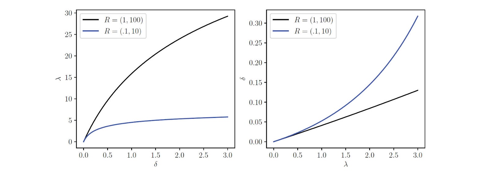
Slope at zero.
Using (16), we see that F'(0^+) = E_{ij}, i.e., the one-sided derivative at 0 is exactly the exchange rate for assets i and j. Since F is concave, we have
(18)F(\delta) \leq F'(0^+)\delta = E_{ij} \delta.
This tells us that the amount of asset j you will receive for trading \delta of asset i is no more than the amount predicted by the exchange rate.
The one-sided derivative of the reverse exchange function G at 0 is G'(0^+) = E_{ji}. The analog of the inequality (18) is
(19)G(\lambda) \geq G'(0^+)\lambda = \gamma^{-2} E_{ji} \lambda,
which states that the amount of asset i you need to tender to receive an amount of asset j is at least the amount predicted by the exchange rate.
Examples.
Figure 1 shows the forward and reverse exchange functions for a constant geometric mean market with two assets and weights w_1 = .2 and w_2 = .8, and \gamma =0.997. We show the functions for two values of the reserves: R=(1,100) and R=(0.1,10). The exchange rate is the same for both values of the reserves and equal to E_{12} = \gamma w_1R_2/w_2R_1 = 25.
4.2. Exchanging multiples of two baskets
Here we discuss a simple generalization of two-asset trade, in which we tender and receive a multiple of fixed baskets. Thus, we have \Delta = \delta \tilde \Delta and \Lambda = \lambda \tilde \Lambda, where \lambda\geq 0 and \delta \geq 0 scale the fixed baskets \tilde \Delta and \tilde \Lambda. When \tilde \Delta = e_i and \tilde \Lambda= e_j, this reduces to the two-asset trade discussed above.
The same analysis holds in this case as in the simple two-asset trade. We can introduce the forward and reverse functions F and G, which are inverses of each other. They are increasing, F is concave, G is convex, and they satisfy F(0)=G(0)=0. We have the inequality F(\delta) \leq E \delta, where E is the exchange rate for exchanging the basket \tilde \Delta for the basket \tilde \Lambda, given by E = \gamma \frac{\nabla \varphi(R)^T \tilde \Delta}{\nabla \varphi(R)^T \tilde \Lambda}. There is also an inequality analogous to (19), using this definition of the exchange rate. We mention two specific important examples in what follows.
Liquidating assets.
Let \Delta\in {{\bf R}}_+^n denote a basket of assets we wish to liquidate, i.e., exchange for the numeraire. We can assume that \Delta_n=0. We then find the \alpha>0 for which (\Delta,\alpha e_n) is a valid trade, i.e.,
(20)\varphi(R+\gamma \Delta - \alpha e_n) = \varphi(R).
We can interpret \alpha as the liquidation value of the basket \Delta . We can also show that the liquidation value is at most as large as the discounted value of the basket; i.e., \alpha \le \gamma p^T\Delta.
To see this, apply (1) to the left hand side of (20), which gives, after cancelling \varphi(R) on both sides, \nabla\varphi(R)^T(\gamma \Delta - \alpha e_n) \ge 0. Rearranging, we find: \alpha \le \frac{\gamma\nabla\varphi(R)^T\Delta}{\nabla\varphi(R)_n} = \gamma p^T\Delta.
Purchasing a basket.
Let \Lambda \in {{\bf R}}_+^n denote a basket we wish to purchase using the numeraire. We find \alpha >0 for which (\alpha e_n,\Lambda) is a valid trade, i.e., \varphi(R+\gamma \alpha e_n - \Lambda) = \varphi(R). We interpret \alpha as the purchase cost of the basket \Lambda. It can be shown that \alpha \geq (1/\gamma) p^T \Lambda, i.e., the purchase cost is at least a factor 1/\gamma more than the value of the basket, at the current prices. This follows from a nearly identical argument to that of the liquidation value.
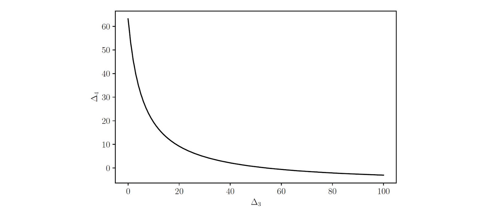
Figure 2: Valid tendered baskets (\Delta3, \Delta4) for the received basket \Lambda = (2,4,0,0).
5. Multi-asset trades
We have seen that two-asset trades are easy to understand; we choose the amount we wish to tender (or receive), and we can then find the amount we will receive (or tender). Multi-asset trade are more complex, because even for a fixed receive basket \Lambda, there are many tender baskets that are valid, and we face the question of which one should we use. The same is true when we fix the tendered basket \Delta: there are many baskets \Lambda we could receive, and we need to choose one. More generally, we have the question of how to choose the proposed trade (\Delta,\Lambda). In the two-asset case, the choice is parametrized by a scalar, either \delta or \lambda. In the multi-asset case, there are more degrees of freedom.
Example.
We consider an example with n=4, geometric mean trading function with weights w_i = 1/4 and fee \gamma = .997, with reserves R = (4, 5, 6, 7). We fix the received basket to be \Lambda = (2,4,0,0). There are many valid tendered baskets, which are shown in figure 2. The plot shows valid values of (\Delta_3, \Delta_4), since the first two components of \Delta are zero.
{#f-tendered width=”.8\\textwidth”}
5.1. The general trade choice problem
We formulate the problem of choosing (\Delta,\Lambda) as an optimization problem. The net change in holdings of the trader is \Lambda - \Delta. The trader judges a net change in holdings using a utility function U:{{\bf R}}^n \to {{\bf R}}\cup\{-\infty\}, where she prefers (\Delta,\Lambda) to (\tilde \Delta, \tilde \Lambda) if U(\Lambda - \Delta)> U(\tilde \Lambda - \tilde \Delta). The value -\infty is used to indicate that a change in holdings is unacceptable. We will assume that U is increasing and concave. (Increasing means that the trader would always prefer to have a larger net change than a smaller one, which comes from our assumption that all assets have value.)
To choose a valid trade that maximizes utility, we solve the problem
(21)\begin{aligned} & \text{maximize} && U(\Lambda - \Delta) \\ & \text{subject to} && \varphi(R+\gamma \Delta - \Lambda) = \varphi(R), \quad \Delta \geq 0, \quad \Lambda \geq 0, \end{aligned}
with variables \Delta and \Lambda. Unfortunately the constraint \varphi(R+\gamma \Delta - \Lambda) = \varphi(R) is not convex (unless the trading function is linear), so this problem is not in general convex.
Instead we will solve its convex relaxation, where we change the equality constraint to an inequality to obtain the convex problem
(22)\begin{aligned} & \text{maximize} && U(\Lambda - \Delta) \\ & \text{subject to} && \varphi(R+\gamma \Delta - \Lambda) \geq \varphi(R), \quad \Delta \geq 0, \quad \Lambda \geq 0, \end{aligned}
which is readily solved. It is easy to show that any solution of (22) satisfies \varphi(R+\gamma \Delta - \Lambda) = \varphi(R), and so is also a solution of the problem (21). (If a solution satisfies \varphi(R+\gamma \Delta - \Lambda) > \varphi(R), we can decrease \Delta or increase \Lambda a bit, so as to remain feasible and increase the objective, a contradiction.)
Thus we can (globally and efficiently) solve the non-convex problem (21) by solving the convex problem (22).
No-trade condition.
Assuming U(0) > - \infty, the solution to the problem (22) can be \Delta = \Lambda = 0, which means that trading does not increase the trader’s utility, i.e., the trader should not propose any trade. We can give simple conditions under which this happens for the case when U is differentiable. They are
(23)\gamma p \leq \alpha\nabla U(0) \leq p,
for some \alpha>0. We can interpret the set of prices p for which this is true, i.e., K = \{p \in {{\bf R}}^n_+ \mid \gamma p \le \alpha \nabla U(0) \le p ~ \text{for some} ~ \alpha > 0\}, as the no-trade cone for the utility function U. (It is easy to see that K is a convex polyhedral cone.)
We interpret \nabla U(0) as the vector of marginal utilities to the trader, and p as the prices of the assets in the CFMM. For \gamma =1, the condition says that we do not trade when the marginal utility is a positive multiple of the current asset prices; if this does not hold, then the solution of the trading problem (22) is nonzero, i.e., the trader should trade to increase her utility. When \gamma<1, the trader will not trade when the prices are in K.
To derive condition (23), we first derive the optimality conditions for the problem (22). We introduce the Lagrangian L(\Delta, \Lambda, \lambda, \omega, \kappa) = U(\Lambda -\Delta) + \lambda(\varphi(R+\gamma \Delta-\Lambda)-\varphi(R)) + \omega^T\Delta + \kappa^T\Lambda, where \lambda \in {{\bf R}}_+, \omega\in {{\bf R}}_+^n, and \kappa \in {{\bf R}}_+^n are dual variables or Lagrange multipliers for the constraints. The optimality conditions for (22) are feasibility, along with \nabla_\Delta L = 0, \qquad \nabla _\Lambda L = 0. The choice \Delta=0, \Lambda =0 is feasible, and satisfies this condition if \nabla_\Delta L(0,0,\lambda,\omega,\kappa) = 0, \qquad \nabla_\Lambda L(0,0,\lambda,\omega,\kappa) = 0. These are - \nabla U(0) + \lambda \gamma \nabla \varphi(R) + \omega =0, \qquad \nabla U(0) - \lambda \nabla \varphi(R) + \kappa=0, which we can write as \nabla U(0) \geq \lambda \gamma \nabla \varphi(R), \qquad \nabla U(0) \leq \lambda \nabla \varphi(R). Dividing these by \lambda P_n, we obtain (23) with \alpha = 1/(\lambda P_n).
5.2. Special cases
Linear utility.
When U(z) = \pi^T z, with \pi \geq 0, we can interpret \pi as the trader’s private prices of the assets, i.e., the prices she values the assets at. From (23) we see that the trader will not trade if her private asset prices satisfy
(24)\gamma p \le \alpha\pi \le p
for some \alpha > 0.
In the special case where \pi satisfies (\pi_2, \dots, \pi_n) = \lambda (p_2, \dots, p_n), for \lambda \ge 0, i.e., \pi is collinear with p except in the first entry, (24) is satisfied if and only if \lambda \gamma p_1 \le \pi_1 \le \lambda \gamma^{-1}p_1. If \lambda = 1, then this simplifies to the condition \gamma p_1 \le \pi_1 \le \gamma^{-1}p_1. (This will arise in an example we present below.)
Markowitz trading.
Suppose the trader models the return r\in {{\bf R}}^n on the assets over some period of time as a random vector with mean \mathop{\bf E{}}r = \mu \in {{\bf R}}^n and covariance matrix \mathop{\bf E{}}(r-\mu)(r-\mu)^T =\Sigma \in {{\bf R}}^{n\times n}. If the trader holds a portfolio of assets z \in {{\bf R}}^n_+, the return is r^T z; the expected portfolio return is \mu^Tz and the variance of the portfolio return is z^T\Sigma z. In Markowitz trading, the trader maximizes the risk-adjusted return, defined as \mu^T z - \kappa z^T\Sigma z, where \kappa>0 is the risk-aversion parameter6263. This leads to the Markowitz trading problem
(25)\begin{aligned} & {maximize} && \mu^T z - \kappa z^T \Sigma z\\ &{subject to} && z = z^\text{curr} - \Delta + \Lambda \\ &&&\varphi(R+\gamma \Delta - \Lambda) \geq \varphi(R)\\ &&& \Delta \geq 0, \quad \Lambda \geq 0, \end{aligned}
with variables z, \Delta, \Lambda, where z^\text{curr} is the trader’s current holdings of assets. This is the general problem (22) with concave utility function U(Z) = \mu^T(z^\text{curr} + Z) - \kappa (z^\text{curr} + Z)^T \Sigma (z^\text{curr} + Z).
A well-known limitation of the Markowitz quadratic utility function U, i.e., the risk-adjusted return, is that it is not increasing for all Z, which implies that the trading function relaxation need not be tight. However, for any sensible choice of the parameters \mu and \Sigma, it is increasing for the values of Z found by solving the Markowitz problem (25), and the relaxation is tight. As a practical matter, if a solution of (25) does not satisfy the trading constraint, then the parameters are inappropriate.
Expected utility trading.
Here the trader models the returns r\in {{\bf R}}^m on the assets over some time interval as random, with some known distribution. The trader seeks to maximize the expected utility of the portfolio return, using a concave increasing utility function \psi: {{\bf R}}\to {{\bf R}} to introduce risk aversion. (Thus we use the term utility function to refer to both the trading utility function U: {{\bf R}}_+^n \to {{\bf R}} and the portfolio return utility function \psi:{{\bf R}}\to {{\bf R}}, but the context should make it clear which is meant.) This leads to the problem
(26)\begin{aligned} & {maximize} && \mathop{\bf E{}}\psi(r^Tz)\\ &{subject to} && z = z^\text{curr} - \Delta + \Lambda \\ &&&\varphi(R+\gamma \Delta - \Lambda) \geq \varphi(R)\\ &&& \Delta \geq 0, \quad \Lambda \geq 0, \end{aligned}
where the expectation is over r. This is the general problem (22), with utility U(Z) = \mathop{\bf E{}}\psi (r^T (z^\text{curr}+Z)), which is concave and increasing.
This problem can be solved using several methods. One simple approach is to replace the expectation with an empirical or sample average over some Monte Carlo samples of r, which leads to an approximate solution of (26). The problem can also be solved using standard methods for convex stochastic optimization, such as projected stochastic gradient methods.
5.3. Numerical examples
In this section we give two numerical examples.
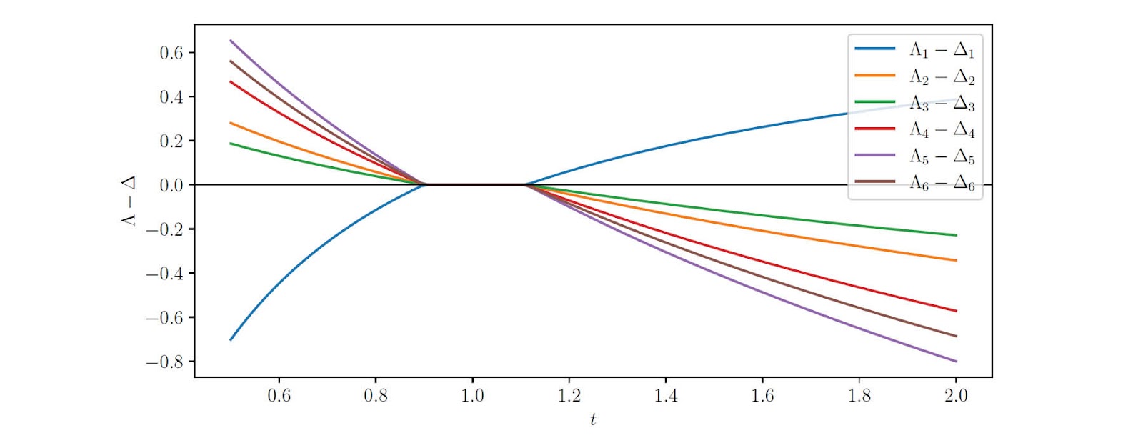
Figure 3: Solutions \Lambda - \Delta for the linear utility maximization problem, as the private price for asset 1 is varied by the factor t from the CFMM price. The blue curve shows asset 1.
Linear utility.
Our first example involves a CFMM with 6 assets, geometric mean trading function with equal weights w_i = 1/6, and trading fee parameter \gamma = .9. (We intentionally use an unrealistically small value of \gamma so the no-trade condition is more evident.) We take reserves R = (1, 3, 2, 5, 7, 6). The corresponding prices are given by (9), p = (R_6/R_1, R_6/R_2, \ldots, 1) = (6, 2, 3, 6/5, 6/7, 1). We consider linear utility, with the trader’s private prices given by \pi = (tp_1, p_2, \dots, p_n), where t is a parameter that we vary over the interval t \in [1/2,2]. For t=1, we have \pi=p, i.e., the CFMM prices and the trader’s private prices are the same (and not surprisingly, the trader does not trade). As we vary t, we vary the trader’s private price for asset 1 by up to a factor of two from the CFMM price.
The family of optimal trades are shown in figure 3, as a function of the parameter t. We plot \Lambda - \Delta versus t, which shows assets in the tender basket as negative and the received basket as positive. The blue curve shows asset 1, which we tender when t is small, and receive when t is large. The no-trade region is clearly seen as the interval t\in [0.9,1.1].
Markowitz trading.

Figure 4: Solutions \Lambda - \Delta for instances of an example Markowitz trading problem as the risk-aversion parameter \kappa is varied.
Our second example uses nearly the same CFMM and reserves as the previous example, but with a more realistic trading fee parameter \gamma = .997. (This is a common choice of trading fee for many CFMMs.) We solve the Markowitz trading problem (25), with current holdings z^\text{curr} = (2.5, 1, .5, 2.5, 3, 1), mean return \mu = (-.01, .01, .03, .05, -.02, .02), and covariance \Sigma = V^TV/100, where the entries of V\in {{\bf R}}^{6\times 6} are drawn from the standard normal distribution. We solve the optimal trading problem for values of the risk aversion parameter \kappa varying between 10^{-2} and 10^{1}. (For all of these values, the trading constraint is tight.) These optimal trades are shown in figure 4. It is interesting to note that depending on the risk aversion, we either tender or receive assets 2 and 3.
The CVXPY code for the Markowitz optimal trading problem is given below. In this snippet we assume that `mu`, `sigma`, `gamma`, `kappa`, `R`, and `z_curr` have been previously defined. Note that the code closely follows the mathematical description of the problem given in (25).
6. Conclusion
We have provided a general description of CFMMs, outlining how users can interact with a CFMM through trading or adding and removing liquidity. We observe that many of the properties of CFMMs follow from concavity of the trading function. In the simple case where two assets are traded or exchanged, it suffices to specify the amount we wish to receive (or tender), which determines the amount we tender (receive), by simply evaluating a convex (concave) function. Multi-asset trades are more complex, since the set of valid trades is multi-dimensional, i.e., multiple tender or received baskets are possible. We formulate the problem of choosing from among these possible valid trades as a convex optimization problem, which can be globally and efficiently solved.

Listing 1: Markowitz trading CVXPY code.
Acknowledgements
The authors would like to acknowledge Shane Barratt for useful discussions. Guillermo Angeris is supported by the National Science Foundation Graduate Research Fellowship under Grant No. DGE-1656518. Akshay Agrawal is supported by a Stanford Graduate Fellowship.
References
- Michael Egorov. StableSwap – efficient mechanism for Stablecoin liquidity. page 6, 2019. [↩] [↩] [↩]
- Yi Zhang, Xiaohong Chen, and Daejun Park. Formal specification of constant product (xy = k) market maker model and implementation. 2018. [↩] [↩] [↩]
- Hayden Adams, Noah Zinsmeister, Moody Salem, River Keefer, and Dan Robinson. Uniswap v3 core. Technical report, 2021. [↩] [↩]
- Sushi. The SushiSwap project, 2020. [↩] [↩] [↩]
- Alan Lu. Building a decentralized exchange in Ethereum. https://blog.gnosis.pm/building-a-decentralized-exchange-in-ethereumeea4e7452d6e, 2017. [↩]
- Vitalik Buterin. On path independence. https://vitalik.ca/general/2017/06/22/marketmakers.html, 2017. [↩]
- Yi Zhang, Xiaohong Chen, and Daejun Park. Formal specification of constant product (xy = k) market maker model and implementation. 2018. [↩]
- Fernando Martinelli and Nikolai Mushegian. Balancer: A non-custodial portfolio manager, liquidity provider, and price sensor. 2019. [↩] [↩]
- Guillermo Angeris and Tarun Chitra. Improved price oracles: Constant function market makers. In Proceedings of the 2nd ACM Conference on Advances in Financial Technologies, pages 80–91, New York NY USA, October 2020. ACM. [↩] [↩] [↩]
- Stephen Boyd and Lieven Vandenberghe. Convex Optimization. Cambridge University Press, Cambridge, UK ; New York, 2004. [↩] [↩] [↩] [↩]
- Satoshi Nakamoto. Bitcoin: A peer-to-peer electronic cash system, 2008. [↩]
- Vitalik Buterin. Ethereum: A next-generation smart contract and decentralized application platform, 2013. [↩]
- Gavin Wood. Ethereum: A secure decentralised generalised transaction ledger, 2014. [↩]
- Gavin Wood. Polkadot: Vision for a heterogeneous multi-chain framework, 2016. [↩]
- Anatoly Yakovenko. Solana: A new architecture for a high performance blockchain, 2018. [↩]
- Nick Szabo. Smart contracts. Extropy: Journal of Transhumanist Thought, 16, 1995. [↩]
- Aave. https://aave.com, 2021. [↩]
- Compound. https://compound.finance, 2021. [↩]
- UMA project. https://umaproject.org, 2021. [↩]
- dydx. https://dydx.exchange, 2021. [↩]
- Robert Winkler. Scoring rules and the evaluation of probability assessors. Journal of the American Statistical Association*, 64(327):1073–1078, 1969.30 [↩]
- Robin Hanson. Combinatorial information market design. *Information Systems Frontiers*, 5(1):107–119, 2003. [↩]
- Yiling Chen, Lance Fortnow, Nicolas Lambert, David Pennock, and Jennifer Wortman. Complexity of combinatorial market makers. In Proceedings of the 9th ACM Conference on Electronic Commerce, pages 190–199, 2008. [↩]
- Guillermo Angeris, Hsien-Tang Kao, Rei Chiang, Charlie Noyes, and Tarun Chitra. An analysis of Uniswap markets. *Cryptoeconomic Systems*, November 2020. [↩]
- Alex Evans. Liquidity provider returns in geometric mean markets. arXiv preprint arXiv:2006.08806, 2020. [↩]
- Guillermo Angeris, Alex Evans, and Tarun Chitra. Replicating market makers. arXiv preprint arXiv:2103.14769, 2021. [↩]
- Alex Evans, Guillermo Angeris, and Tarun Chitra. Optimal fees for geometric mean market makers. arXiv preprint arXiv:2104.00446, 2021. [↩]
- Martin Tassy and David White. Growth rate of a liquidity provider’s wealth in xy = c automated market makers, 2020. [↩]
- Guillermo Angeris, Alex Evans, and Tarun Chitra. When does the tail wag the dog? Curvature and market making. arXiv preprint arXiv:2012.08040, 2020. [↩]
- Jun Aoyagi. Liquidity provision by automated market makers. Available at SSRN 3674178, 2020. [↩]
- Jun Aoyagi and Yuki Ito. Liquidity implications of constant product market makers. Available at SSRN 3808755, 2021. [↩]
- Guillermo Angeris, Alex Evans, and Tarun Chitra. A note on privacy in constant function market makers. arXiv preprint arXiv:2103.01193, 2021. [↩]
- Tarun Chitra, Guillermo Angeris, Alex Evans, and Hsien-Tang Kao. A note on borrowing constant function market maker shares. 2021. [↩]
- Ye Wang, Yan Chen, Shuiguang Deng, and Roger Wattenhofer. Cyclic arbitrage in decentralized exchange markets. Available at SSRN 3834535, 2021. [↩]
- Ernest Ryu and Stephen Boyd. A primer on monotone operator methods. Applied Computational Math, 2016. [↩]
- Gregory Stewart and Francesco Borrelli. A predictive control framework for industrial turbodiesel engine control. In IEEE Conference on Decision and Control (CDC), pages 5704–5711, 2008. [↩]
- Lars Blackmore. Autonomous precision landing of space rockets. The BRIDGE, 26(4), 2016. [↩] [↩]
- Thomas Lipp and Stephen Boyd. Minimum-time speed optimisation over a fixed path. International Journal of Control, 87(6):1297–1311, 2014. [↩]
- Gerard Cornuejols and Reha Tu¨tu¨ncu¨. Optimization Methods in Finance. Cambridge University Press, 2006. [↩]
- Stephen Boyd, Enzo Busseti, Steven Diamond, Ronald Kahn, Kwangmoo Koh, Peter Nystrup, and Jan Speth. Multi-period trading via convex optimization. Foundations and Trends in Optimization, 3(1):1–76, 2017. [↩]
- Nicholas Moehle, Enzo Busseti, Stephen Boyd, and Matt Wytock. Dynamic energy management. arXiv preprint arXiv:1903.06230, 2019. [↩]
- Akshay Agrawal, Stephen Boyd, Deepak Narayanan, Fiodar Kazhamiaka, and Matei Zaharia. Allocation of fungible resources via a fast, scalable price discovery method. arXiv preprint arXiv:2104.00282, 2021. [↩]
- Jerome Friedman, Trevor Hastie, and Robert Tibshirani. The Elements of Statistical Learning, volume 1. Springer Series in Statistics, 2001. [↩]
- Stephen Boyd, Neal Parikh, Eric Chu, Borja Peleato, and Jonathan Eckstein. Distributed optimization and statistical learning via the alternating direction method of multipliers. Foundations and Trends©R in Machine learning, 3(1):1–122, 2011. [↩]
- Guillermo Angeris, Jelena Vuˇckovi´c, and Stephen Boyd. Heuristic methods and performance bounds for photonic design. Optics Express, 29(2):2827, January 2021.27 [↩]
- Maria Hershenson, Stephen Boyd, and Thomas Lee. Optimal design of a CMOS op-amp via geometric programming. IEEE Transactions on Computer-aided design of integrated circuits and systems, 20(1):1–21, 2001. [↩]
- Stephen Boyd, Seung-Jean Kim, Dinesh Patil, and Mark Horowitz. Digital circuit optimization via geometric programming. Operations Research, 53(6), 2005. [↩]
- Bartolomeo Stellato, Goran Banjac, Paul Goulart, Alberto Bemporad, and Stephen Boyd. OSQP: An operator splitting solver for quadratic programs. Mathematical Programming Computation, February 2020. [↩] [↩]
- Brendan O’Donoghue, Eric Chu, Neal Parikh, and Stephen Boyd. Conic optimization via operator splitting and homogeneous self-dual embedding. Journal of Optimization Theory and Applications, 169(3):1042–1068, June 2016. [↩]
- Alexander Domahidi, Eric Chu, and Stephen Boyd. ECOS: An SOCP solver for embedded systems. In 2013 European Control Conference (ECC), pages 3071–3076, Zurich, July 2013. IEEE. [↩] [↩]
- Michael Garstka, Mark Cannon, and Paul Goulart. COSMO: A conic operator splitting method for large convex problems. In 2019 18th European Control Conference (ECC), pages 1951–1956, Naples, Italy, June 2019. IEEE. [↩]
- MOSEK ApS. MOSEK Optimizer API for Python 9.1.5. https://docs.mosek.com/9.1/pythonapi/index.html, 2019. [↩]
- Yang Wang and Stephen Boyd. Fast evaluation of quadratic control-Lyapunov policy. IEEE Transactions on Control Systems Technology, 19(4):939–946, 2010. [↩]
- Jacob Mattingley and Stephen Boyd. CVXGEN: A code generator for embedded convex optimization. Optimization and Engineering, 13(1):1–27, 2012. [↩] [↩]
- Eric Chu, Neal Parikh, Alexander Domahidi, and Stephen Boyd. Code generation for embedded second-order cone programming. In European Control Conference, pages 1547–1552. IEEE, 2013. 28 [↩]
- Goran Banjac, Bartolomeo Stellato, Nicholas Moehle, Paul Goulart, Alberto Bemporad, and Stephen Boyd. Embedded code generation using the OSQP solver. In IEEE Conference on Decision and Control, 2017. [↩]
- Steven Diamond and Stephen Boyd. CVXPY: A Python-embedded modeling language for convex optimization. Journal of Machine Learning Research, 17(83):1–5, 2016. [↩]
- Akshay Agrawal, Robin Verschueren, Steven Diamond, and Stephen Boyd. A rewriting system for convex optimization problems. Journal of Control and Decision, 5(1):42–60, 2018. [↩]
- Iain Dunning, Joey Huchette, and Miles Lubin. JuMP: A modeling language for mathematical optimization. SIAM review, 59(2):295–320, 2017. [↩]
- Guillermo Angeris, Hsien-Tang Kao, Rei Chiang, Charlie Noyes, and Tarun Chitra. An analysis of Uniswap markets. Cryptoeconomic Systems, November 2020. [↩]
- William Press, Saul Teukolsky, Brian Flannery, and William Vetterling. Numerical Recipes: The Art of Scientific Computing. Cambridge University Press, 1992. §9 [↩]
- Harry Markowitz. Portfolio selection. The Journal of Finance, 7(1):77–91, 1952. 29 [↩]
- Stephen Boyd, Enzo Busseti, Steven Diamond, Ronald Kahn, Kwangmoo Koh, Peter Nystrup, and Jan Speth. Multi-period trading via convex optimization. Foundations and Trends in Optimization, 3(1):1–76, 2017. [↩]